How to estimate the age of your brain with MRI data - A practical guide for applying machine learning in healthcare

 

 

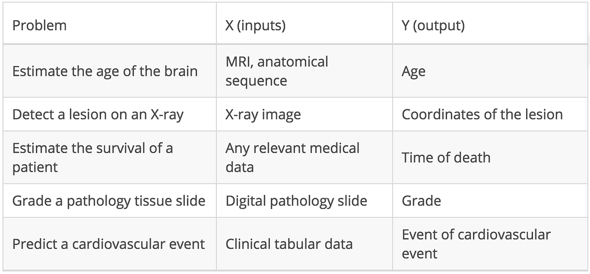
When faced with such problems, data scientists always take a similar approach, no matter the X and Y:

1. Obtain the data and clean it
2. Analyze the data and extract features relevant to the problem
3. Design a validation strategy
4. Train an algorithm on the data, analyze the errors, and interpret the results
5. Iterate until the algorithm is performing the best.

Note: In this work, we used Python, one of the most popular programming language in machine learning. For newcomers, we invite you to execute the first lines of code in the Colab notebook to get a glimpse of how it works.

Data Collection

For this project, we used two publicly available and anonymized datasets of brain MRIs from healthy subjects. The first, Dataset A, was collected in three different London hospitals and contains data from nearly 600 subjects. The second, Dataset B, contains data from more than 1,200 subjects from 25 hospitals across the US, China, and Germany.

Note: This part was easy for us, as the image datasets we used were already collected and curated, as well as usable, from a legal and regulatory perspective. Also medical imaging benefits from having a standard format called DICOM, unlike electronic health records, genomics data, or digital pathology. However, medical dataset compilation is usually the most difficult and time consuming task for physicians and researchers, often taking months to compile data from a few hundred of patients.

As in any data science project,this one began with data cleaning. This begets trouble: ID problems, missing rows within a spreadsheet, low quality images, etc. Such errors are quite common for medical datasets.

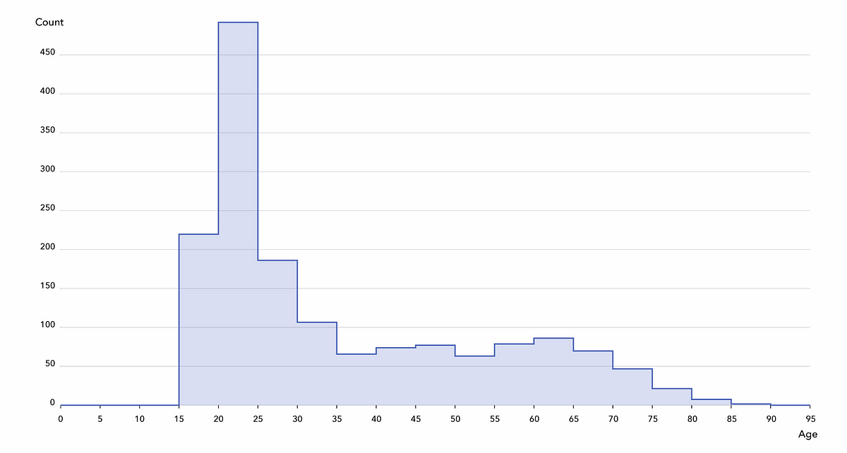
Afterwards, we obtained 563 “clean” subjects from Dataset A (down from 600, 94%) and 1,034 subjects for Dataset B (down from 1,200, 86%). This is captured in the Colab notebook. We observe the following demographics in the cohort: 55% are women, the youngest is 18 years old, the oldest is 87 years old, and quartiles are at 22, 27, and 48.

Data Preprocessing

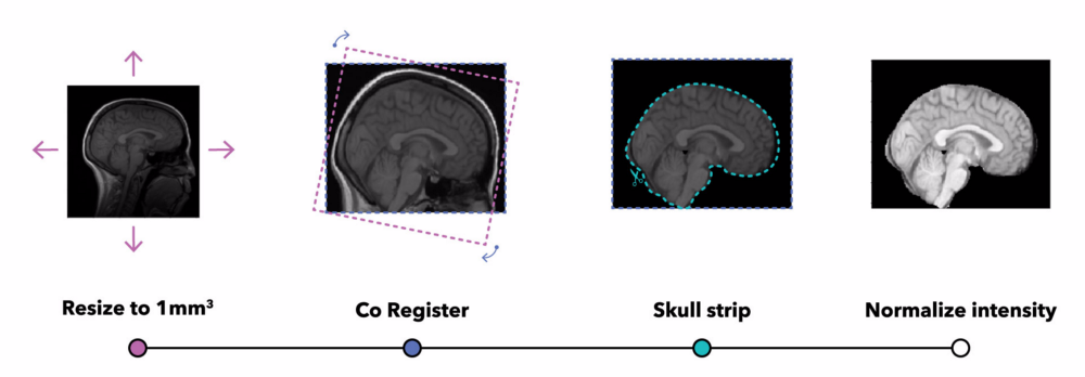
When opening the files containing the MRIs, we observe very high differentiation among the images: resolutions, voxel values, field of view, orientation, etc. Therefore, some method of normalization is needed so we can compare.

Note: The neuroscience and medical imaging communities have developed brain MRI normalization software tools. We applied these, first using ANTs to coregister all images to an atlas (MNI152) and skull strip them, and then normalizing the intensity values of the voxels by applying N4 bias field correction and a popular technique, white stripe normalization. MRI is not a quantitative image, so only contrast matters.

What do doctors know about brain aging?

It is impossible for physicians to determine the precise age of the subject from brain image alone. However, radiologists know at least three anatomical features associated with brain aging, visible on the MRI T1 sequence we used in this work:

• Atrophy, a decrease of the thickness of grey matter (due to loss of neurons)
• Leukoaraiosis, which appears as white matter hypointensities (due to vascular aging)
• Ventricle dilation, as consequence of atrophy and a buildup of cerebrospinal fluid in the brain ventricles.

 

Several researchers have already investigated brain age prediction with anatomical data, as well as its link with brain disorders or genetics. James Cole, a research fellow at King’s College London, has written an excellent series of papers on the topic (Cole et al., 2017 is the most similar to our work). A much larger study (Kaufmann et al., 2018) on around 37,000 patients is currently under review, and both are nicely covered in this Quanta article.

#2 ILLUSTRATING FUNDAMENTALS WITH BRAIM MRI

Starting with a baseline

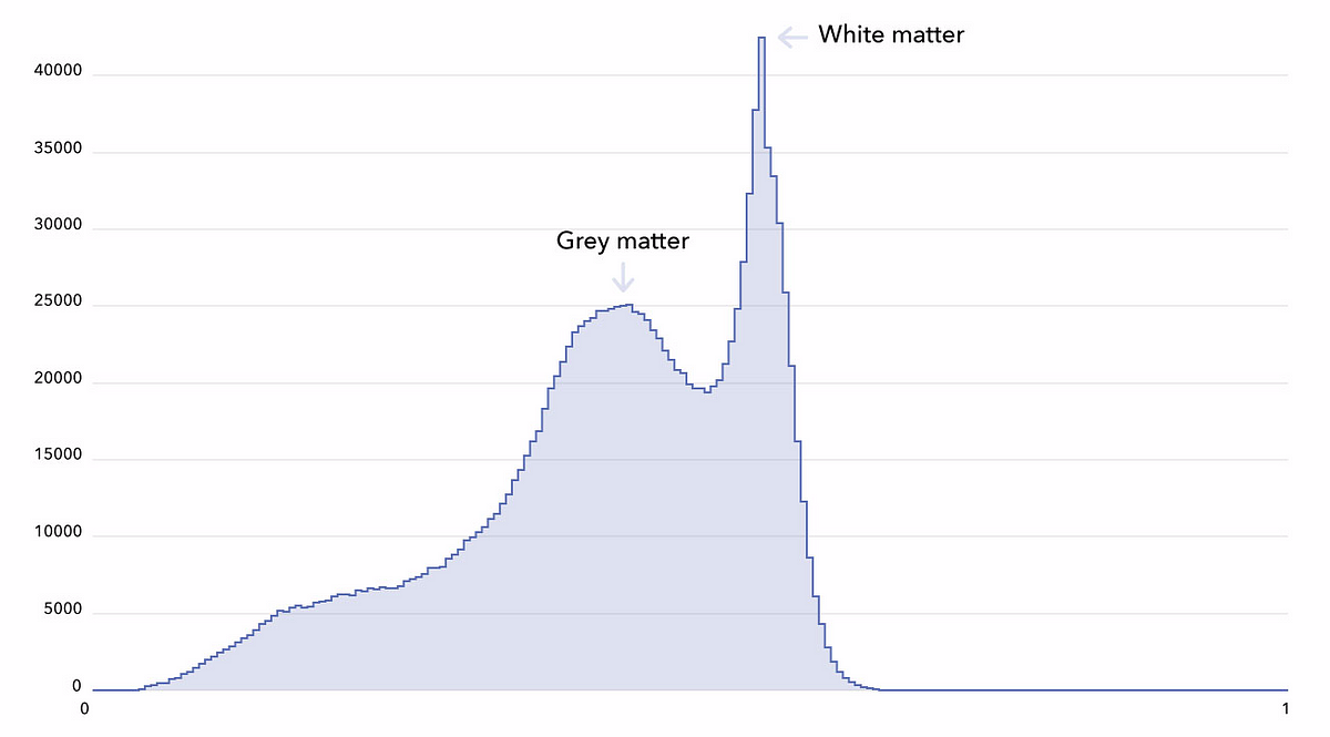
In order to grasp the complexity of the problem,we defined a simple baseline algorithm. We decided to not use the whole 3D MRIs, but instead a simpler reflection of their content, a histogram of their voxel intensities. A typical T1-MRI histogram is shown below (build yours in the Colab notebook).

 

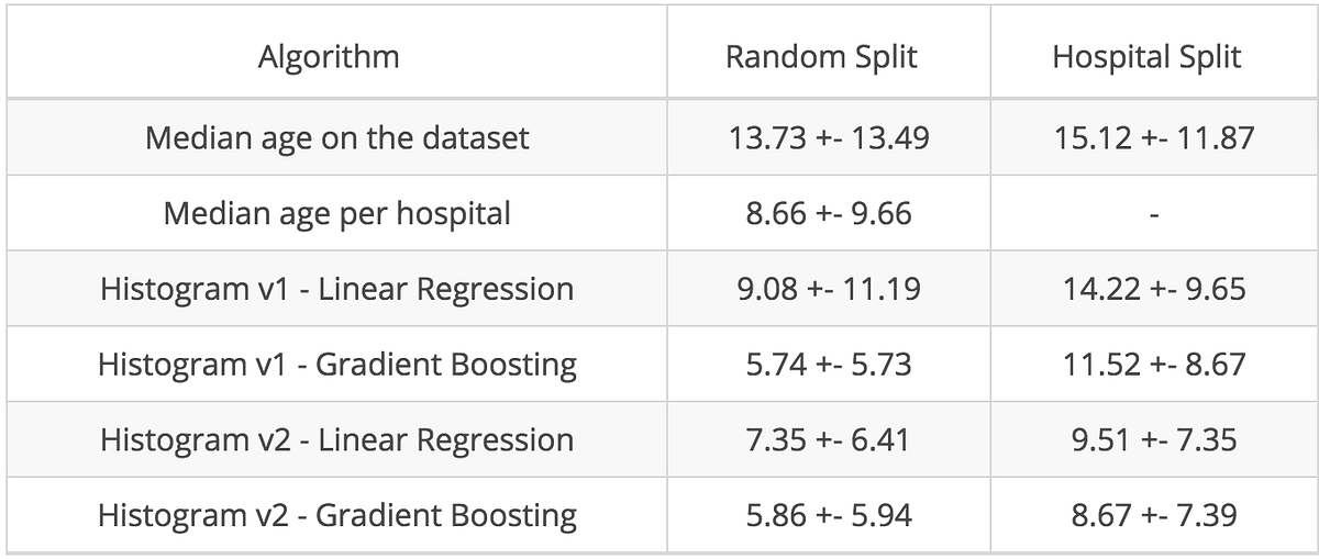
A linear ridge regression trained on these histograms gave us an average mean absolute error of 9.08 years (using a 5-fold cross-validation, random splits). Gradient boosted trees delivered much better results and reduced the error to 5.71 years, which is much closer to state-of-the art performance (4.16 years as reported in Cole et al. 2017). State-of-the-art is a tempting stopping point, but we were making an enormous mistake which is, unfortunately, quite common.

Revisiting the cross validation

The range of the voxels’ intensities in MRIs has no biological meaning and varies greatly from one MRI scanner to another. In the cross-validation procedure, we randomly split subjects between the training and the test set. However, what would be the consequence of randomizing not the subjects but the hospitals, and therefore the MRI scanners?

Once we split by hospital, (with the additional constraint of having a roughly constant training set size), the mean absolute error of our linear regression and gradient boosted trees models increased dramatically by around 5 and 6 years.

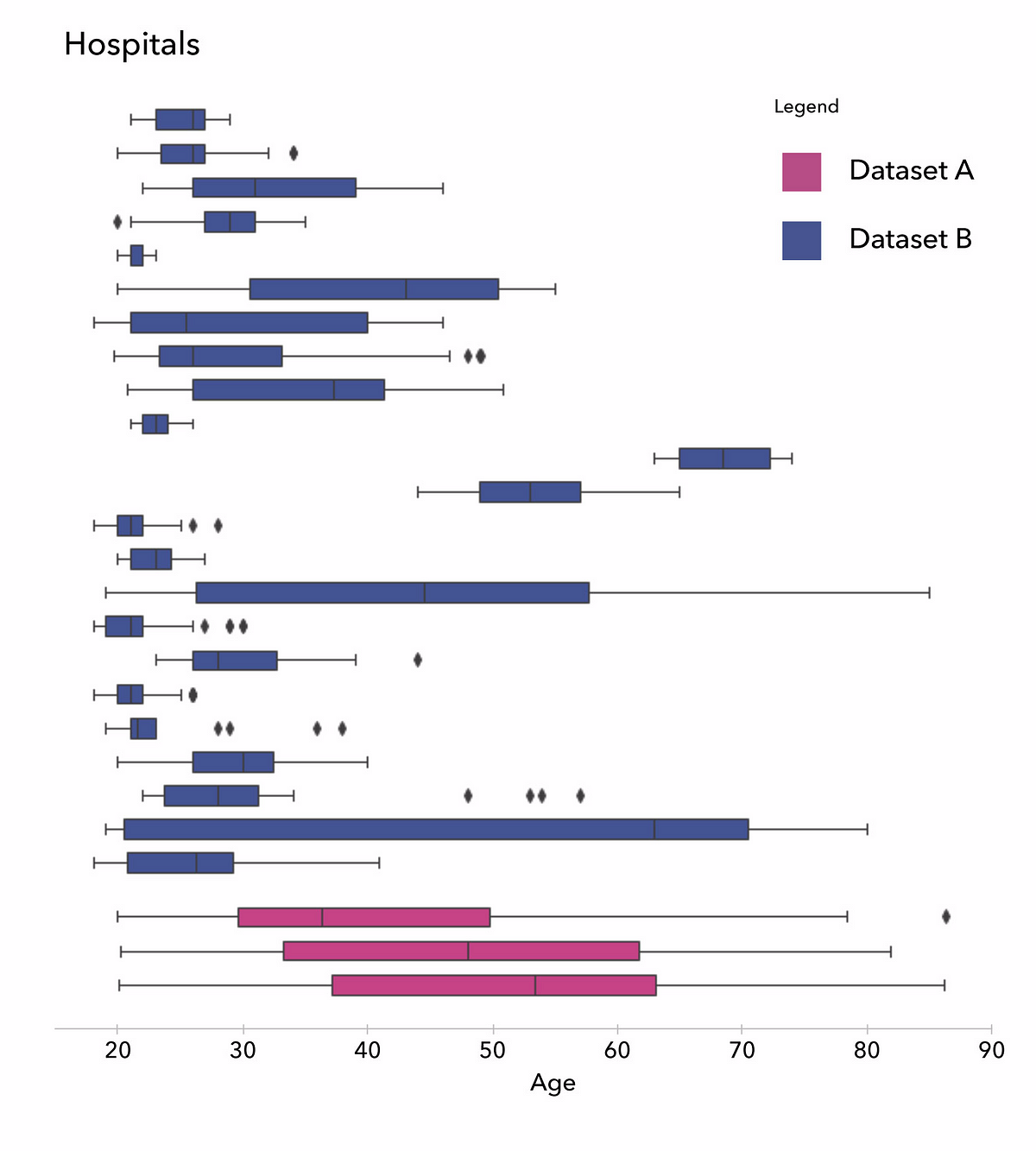
The following two figures show that a more careful data analysis would have prevented us from making such a mistake. In the first one, you can see that the distribution of the ages per hospital are very different: some have only young subjects in their datasets, others only old ones.

 

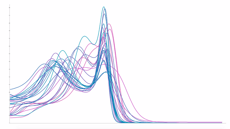
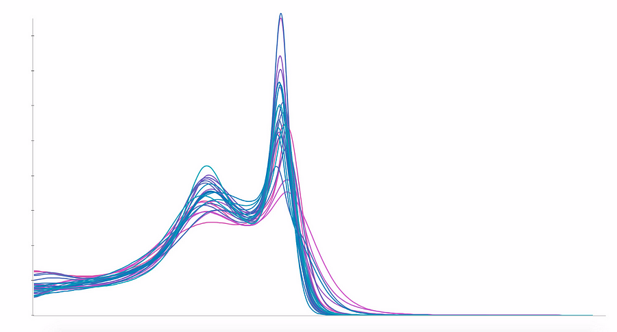
In the next figure, on the left, we show the averaged histograms of the subjects in each hospital and get our explanation : while white matter peaks are quite aligned across different hospitals, grey matter peaks are spread widely. This heterogeneity is generating biases learnable by the algorithms, and may cause misleading predictions. To cancel this effect, we used a homemade normalization method to fix the grey matter peak, as seen below on the right:

As one would expect, the error of the random cross-validation increased with this new normalization, but decreased for the hospital cross-validation, as illustrated below:

 

This section highlighted that cross-validation has to be carefully stratified to avoid including confusion variables (such as an MRI scanner). In our opinion, the best practice for validating an algorithm is to test it on an external and prospective dataset. A bottleneck for inferring truth from evidence-based medicine is the lack of external validity of results in a scientific paper. This can lead, in machine learning vernacular , to a lack of “generalizability” of algorithms.

The concept of “level of evidence” in medicine allows to hierarchize the level of confidence to a given result published in peer-review papers. There is no equivalent today in machine learning.

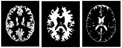
Going further with tissue segmentation

By reducing the entire MRI to a histogram, we ignored spatial information about brain structure. As a next step towards a more effective and interpretable algorithm, we used another software package, FSL FAST, to segment each MRI into grey matter, white matter, and cerebrospinal fluid (CSF). The segmentation is based on the voxel values and yields convincing results that you can explore in our Colab notebook.

 

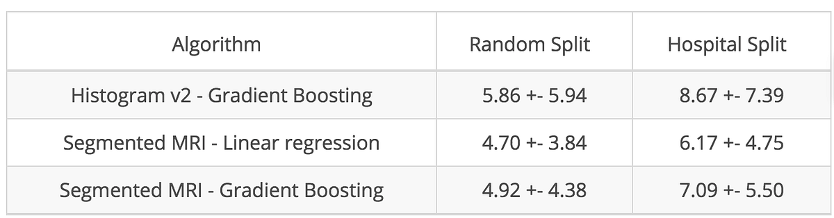
Based on these segmentations, we observed a negative Pearson correlation between age and grey matter total volume of -0.75, confirming the grey matter atrophy hypothesis. Going further, we computed local volumes of the segmented tissues and used them as input of a linear model. Using these expert features, we got better results than with our simple histograms, as illustrated below:

 

#3 GOING BEYOND : EXPLAINABLE DEEP LEARNING 

Let’s start with CNN!

This is the last step of our journey. So far, we manipulated data to extract features we deemed relevant to age prediction. Deep learning takes another approach and uses a family of functions called Convolutional Neural Networks (CNN) which work directly on raw images. They are able to identify the most relevant features for a given task without human guidance.

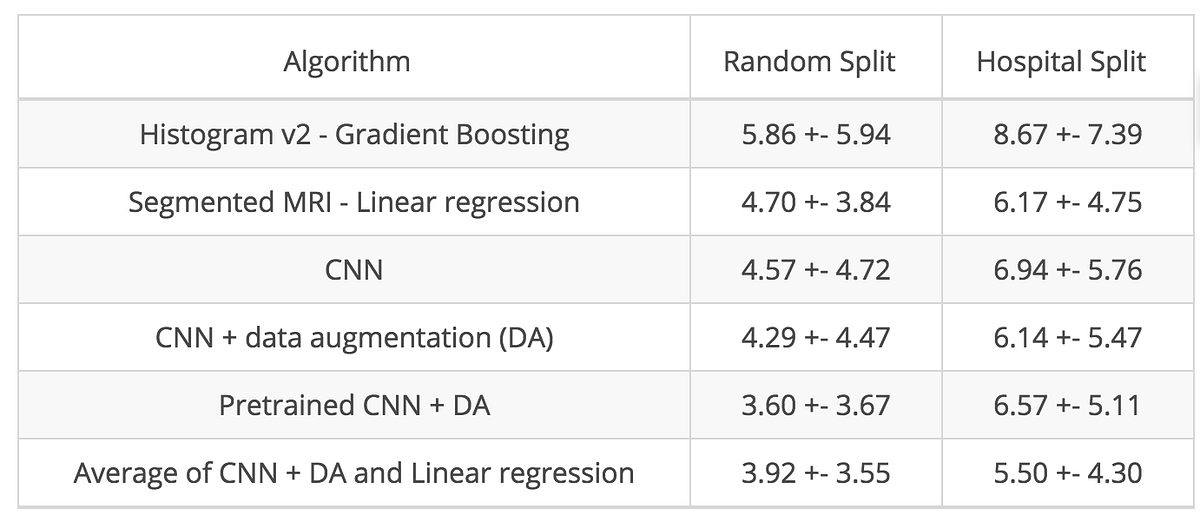
For this case study, we simplified the problem by reducing each MRI from around 200 images in the axial dimension to only 10 images, each representing a 1mm axial zone at the level of the ventricles, where atrophy, ventricle dilation, and leukoaraiosis can be detected. We designed a simple CNN (10 convolutional layers, 5M parameters), obtaining a mean absolute error of 4.57 years for the random split and 6.94 years for the hospital split.

We then improved our models using data augmentation which consists of simulating more data than you have by slightly deforming your dataset, adding small distortions through rotation, zoom, changing intensities of pixels. The trained model can be loaded and used in the Colab notebook.

Transfer learning is a widely-used technique that consists in fine-tuning such pre-trained CNNs on completely new tasks. We used one of these CNNs (ResNet50) and fine-tuned it on our dataset. The complete set of results of these different CNN architectures is represented below:

 

Ensemble methods for the best performance

As a final trick, we averaged the prediction of two of our best algorithms: the CNN with data augmentation and the linear model on the segmented MRI. Comparable to collaboration between experts, ensemble methods bring an additional boost in performance, highlighting that the two models are different but complementary.

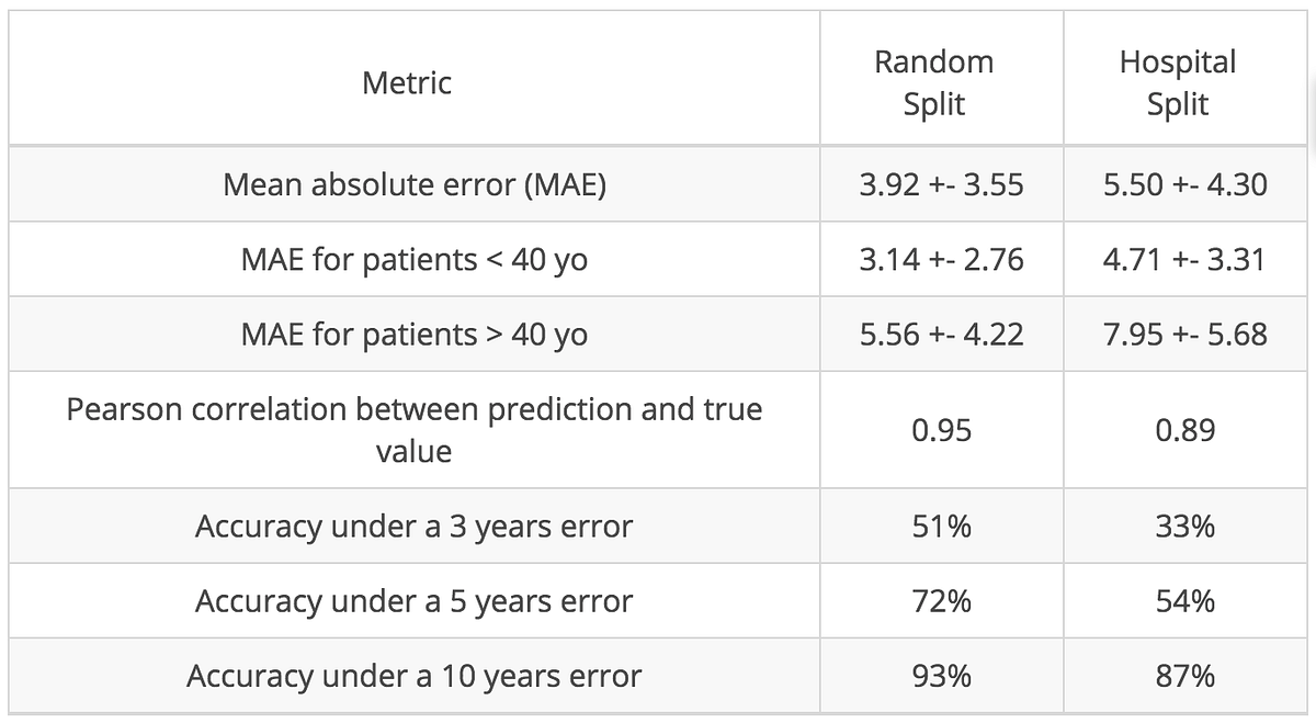
In the table below, we present more metrics of our final model. Because our cohort is young (median age is 27 years old), our model is more reliable for young subjects than for older ones:

 

Looking into the black box

Performance metrics may be convincing but are often not enough to generate trust. Algorithms such as CNNs, with millions of parameters, are difficult to understand and are frustrating black boxes for doctors trying to understand the biology behind the scenes.

As a first glimpse into the black box, we used a simple occlusion technique. The idea was to occlude a small area (4 cm² here) of the test set images and observe the corresponding drop in mean absolute error. If the performance drops significantly , it means that the occluded area was important for the algorithm. On the figure below, the pink regions are associated with the highest error drops:

 

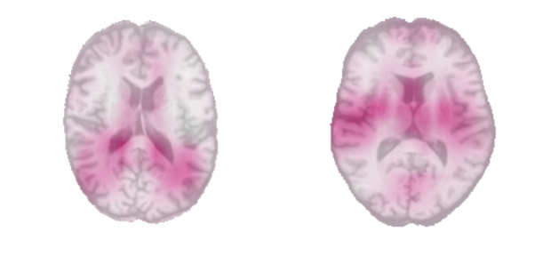
The occlusion map of the youngest subjects on the left revealed that regions closest to the ventricles were important in the prediction, and scientifically, this holds up. We know that ventricles are the thinnest in younger people, as they dilate with aging. The occlusion map of the oldest subjects revealed the importance of the insula on both sides which is consistent with results of Good et al., 2001.

Several more sophisticated techniques to interpret deep learning algorithms are nicely summarized in this post.

Using our model to predict Alzheimer’s disease

The practical application of this exercise is estimating the physiological age of the brain in order to to develop a better understanding of neurodegenerative diseases such as Alzheimer’s disease. As a final experiment, we applied our models on 489 subjects from the ADNI database, split into two categories: normal control (269 subjects) and Alzheimer’s disease (220 subjects).

We downloaded the data, cleaned it, passed it through our preprocessing pipeline, and applied the trained linear regression and CNN models. Patients in this database were much older (averaging 75 years of age) than in the dataset we used for training (averaging 35 years of age), and as one would expect, our models consistently underestimated the age of healthy subjects. This failure highlights an important limitation of machine learning models: if they are not trained on a representative sample of the population, they may perform very badly on unseen subjects. This lack of transferability and the non-stationarity of healthcare data may be one of the most serious hindrances in using machine learning in healthcare.

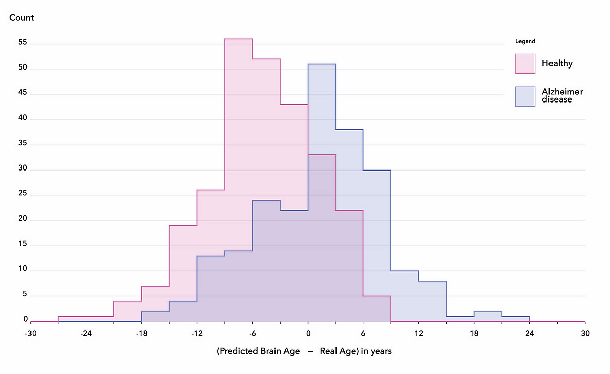
However,, when plotting the distributions of the differences between the reported subject age and the brain age predicted with the final algorithm, we found an average difference of 6 years between patients with Alzheimer’s disease and healthy subjects, corresponding to a ROC-AUC score of 76%. This tends to confirm that the brains of subjects with Alzheimer’s disease somehow contain features correlated to accelerated brain aging (Gaser et al., 2013), corroborating the hypothesis that brain age could be a new biomarker for neurodegenerative diseases (Rafel et al., 2017, Koutsouleris et al., 2014, Coleet al., 2015).

Conclusions

The journey of prediction with machine learning can go from deploying simple linear models in seconds to building complex CNNs that train over days. In both cases, interpretability is crucial, particularly in medicine where it can lead to the discovery of new biological mechanisms or biomarkers.

However, practitioners must be careful when building and analyzing these models. Even when cross-validation is properly stratified, stellar performance on a limited number of use cases does not guarantee good generalization capabilities. This is especially true if the algorithm was not trained on a representative sample of the overall population, and biases are frequent in practice. While difficult from a regulatory and organizational perspective, investing time collecting and cleaning datasets is key for the success of machine learning projects. We hope that this article has given you a taste of what AI looks like when applied to medical data, and has helped you understand common pitfalls to avoid.

Acknowledgements

Several members of the Owkin team contributed to this work, including Simon Jégou*, Paul Herent*, Olivier Dehaene and Thomas Clozel. We thank Dr. Roger Stupp, Dr. Julien Savatovsky, and Olivier Elemento, PhD, for their active support, Sylvain Toldo and Valentin Amé for their work on the figures, as well as Sebastian Schwarz, Eric Tramel, Cedric Whitney, Charlotte Paut and Malika Cantor, for their edits on the manuscript. A longer version of this post is available here

• Simon Jégou, data scientist: simon.jegou@owkin.com
• Paul Herent, radiologist: paul.herent@owkin.com

Check out Owkin website: owkin.com